Dynamics of Gyroscope
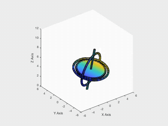
Gyroscope Motion Simulation
For the past few days, I have been working on a group project which is focused on modelling, simulating and animating the dynamic system of a gyroscope. The gyroscope used is composed of two rigid bodies, the frame and the rotor. The system has four degrees of freedom, since the frame can rotate about $x, y, z$ axes, while the rotor can only rotate about the rotor shaft.
Procedure of Analysis
- Record video of gyroscope motion
- Developing the theoretical equations of motion
- MATLAB coding for gyroscope animation (animation output shown at the start)
- Choose model parameters and initial condition to match recording from step 1
The most interesting parts are within step 2 and 3, as there are many procedures required to obtain the equations of motion, which are used for producing the MATLAB animation.
Finding the Equations of Motion
Rotation matrices were defined first to allow clear transition between all the frames. Then other auxiliary variables were defined, so they can be used to find the linear Newton-Euler equations and angular Newton-Euler equations for the gyroscope frame and rotor.
\[\sum F_{object} = m_{object} \cdot \ddot{r}_{OG}\] \[\sum M_{object}^G = \dot{h}_{object}^G\]$G$ is the centre of mass of the object and
\[^{f}\dot{h}_{object}^G = ^{f}h_{object}^{G\prime} + ^{f}\omega_{f} \times ^{f}h_{object}^{G}\] \[^{f}h_{object}^G = ^{f}I^G \cdot ^{f}\omega_{f}\]$f$ is the frame which the calculation is taking place. The prime symbol denotes taking derivative with respect to time.
In the case of analysing the gyroscope rotor, there will be three resulting linear Newton-Euler equations and three angular Newton-Euler equations, which totals to six equations. However, the rotor only has one degree of freedom, therefore there will be one equation of motion for the rotor component. On the other hand, the frame will have three equations of motion because it has three degrees of freedom.
Processing the Equations of Motion
Once the equations of motion are obtained, they can be decoupled and then placed into a pre-defined state vector with matching state equation. These differential equations are solved by using ode45() solver in MATLAB, and evaluated using deval() function. The output values are angles which can be used to map the gyroscope location from the fixed origin.
Animating the Gyroscope Motion
There were some commands which are particularly helpful, including:
cylinderfill3surf
These MATLAB built-in functions allow 3D shapes and geometries to be modelled and created easily. One pending optional objective is to find out how to import existing CAD models into MATLAB for more accurate model representation and simulation.
Ultimately, it was extremely satisfying to see this practical activity from start to end, especially during the moment when all the major bugs are fixed, and the animation starts working.