NIARC Dev Blog 2

Project Update
There has been a significant amount of progress since the previous blog post. From the gif animation above, the robot car can be seen performing the required obstacle avoidance objective for milestone 3. (Might take a little while to load…)
Under the subsections below, I will be going over some of the highlights which have taken place throughout milestone 1 to milestone 3.
Milestone 1
All the team members were able to complete milestone 1 on time, which was regarding the completion of the online NI LabVIEW training course. Although it was not the most interesting nor exciting part of the project, it did allow us to gain a better understanding of LabVIEW itself, hence ensuring that the future milestones can be executed efficiently. This is also a great exercise for practising LabVIEW graphical programming, which is rather different compared other traditional programming languages like C and Java.
Milestone 2
The technical component for milestone 2 was rather simple and straightforward, requiring the team to demonstrate usage of NI myRIO and LabVIEW to control at least one actuator/motor or acquire from at least one sensor.
Since the robot was already assembled, it was rather trivial to write a simple LabVIEW program and record the demo required. However, extra tasks were also completed to better prepare ourselves for the upcoming milestones
However, the project proposal component required more thoughts, as we had to pinpoint most of the critical tasks and the approximate timeline. It is always good to spend more time to plan ahead and minimise any unexpected surprises.
Milestone 3
Right after milestone 2 was completed, the focus quickly shifted to the preparations required for completing milestone 3 - creating a prototype that moves forward and avoiding obstacles. In the following subsections I will be diving into the details regarding the issues faced, how they were resolved and what were completed.
3.1 Reentrancy Issue
Before going into the actual issue, I will try to go over some common terminologies within LabVIEW.
VIis a visual instrument which is like a program and has its own front panel (GUI control elements) and block diagram (where the graphical programming takes place).subVIis like a sub-program, which is not too dissimilar to a function in other programming language. However, they are different in a sense that a subVI can be executed on its own, and can be seen as a VI running within another VI.
This leads to the problem which occurred while implementing and testing some subVIs, as the states of one seemingly independent VI is affecting the output of another VI.
It turns out that it is up to the programmer to configure the reentrancy settings for a VI. The available options are:
- Non-reentrant
- Maintains a single instance of the data space and uses its state across all call sites.
- Lowest memory usage as only a single data space is allocated.
- Shared Clone Reentrancy
- Does not maintain state—Each call site pulls the data space of a clone randomly from the pool of clones. Call sites may end up sharing state.
- Medium memory usage as clones are allocated to accommodate simultaneous instances.
- Preallocated Clone Reentrancy
- Maintains state for each call site—Each call site has its own separate and specific clone.
- Highest memory usage as a clone is allocated for each instance of the subVI.
The problematic behaviour of the program arises from the fact that the same subVI was called with the non-reentrant option selected. The issue was resolved after changing the option to preallocated clone reentrancy. Through this activity, I was able to gain more insight regarding subVI and how they operate.
3.2 PID Control and Tuning
In order to ensure that all the wheels of the robot can turn at the same angular rate of change, PID control implementation is required. Presented below is the time domain form of the PID control equation, where $K_p, K_i, K_d$ refer to the proportional gain, integral gain and derivative gain respectively.
\[u(t) = K_p e(t) + K_i \int_0^t e(\tau) d\tau + K_d \frac{de(t)}{dt}\]The current setup is tuned with the Ziegler-Nichols method which requires the ultimate gain $K_u$ to be found through trial and error. ultimate gain occurs when the motor is just starting to saturate indefinitely. Then we need to find the period of oscillation $T_u$ under the indefinite saturation condition.
After the ultimate gain $K_u$ and period of oscillation $T_u$ are obtained, the following tuning parameters can be applied,
\[u(t) = K_p (e(t) + \frac{1}{T_i}\int_0^t e(\tau)d\tau + T_d \frac{de(t)}{dt})\]and the parameters are defined as follows,
- $K_p = 0.6 K_u$
- $T_i = 0.5 T_u$
- $T_d = 0.125 T_u$
However, this type of tuning method is not thorough and does not encourage an in-depth analysis of the system. It also yields an aggressive gain and overshoot, implying that the perturbed model could easily become unstable, which is evident in the early stages of testing. The gain $K_p$ had to lowered to improve the closed-loop robustness, so that the robot car motors would not saturate during operation.
3.3 Sensor Selection & Evaluation
Since milestone 3 requires the robot car to avoid obstacles, therefore suitable range finding sensors need to be fitted on top of the chassis.
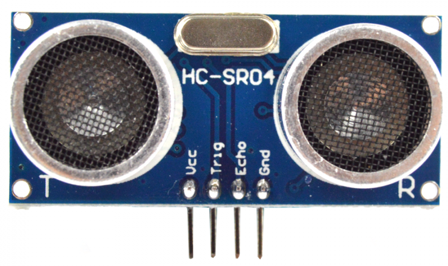
Initially, it was thought that the HC-SR04 ultrasonic sensor would be sufficient for completing milestone 3. However, during the testing and implementation stage, it was discovered that the sensor was rather inaccurate and unreliable. Further filtering is also required to ensure that the sensor readings are usable in operation. Hence, it was decided to look for an alternative.
Note: There is still plan to re-visit this sensor when we are working on signal processing and filtering. It will be fun to see wether it is possible to make this sensor more robust through advanced filtering techniques.
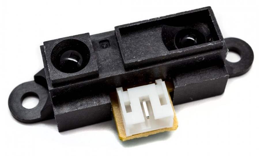
The next sensor considered was the Sharp GP2Y0A21YK0F IR range finder. It turns out that the Sharp IR sensor is more accurate, reliable and easier to use compared to the ultrasonic sensor. Depending on the range of the obstacle in front of the sensor, the IR range finder would return a analog voltage relative to the distance measured. This means that each IR sensor would need to be calibrated manually before installation.
The calibration process is rather straightforward:
- With paper, mark out measured distance on a table.
- Record the output voltage of the sensor at each measured interval (5cm, 10cm, … , 75cm, 80cm).
- Use MATLAB
cftoolto fit a curve through the data points.
The expression of the form,
\[y = a \cdot exp(bx) + c \cdot exp(dx)\]fits the data points rather well. This can be selected within the cftool window by first selecting Exponential and then Number of terms: 2.
3.4 Finite State Machine
After the sensors are calibrated, we are ready to move into the most exciting part of the milestone - programming the robot’s obstacle avoidance algorithm.
Initially, the approach was to use simple if statements (called ‘Case Structures’ in LabVIEW) to make the robot perform simple object avoidance manoeuvre. However, it turns out this approach is really limited in terms of performance and upgradability.
The solution is to program a simple finite state machine in LabVIEW which allows the user to specify as many movement sequences as required, while maintaining the upgradability of the program.
This YouTube Tutorial provides a great overview on finite state machines in LabVIEW and how you can implement one yourself. It also shows you what programming is like in LabVIEW.
What is next?
- Re-designing the robot chassis