NIARC Dev Blog 3
Project Update
The whole project was re-evaluated since the official tasks and rules specified that this year’s competition theme is centred around high-speed rough terrain obstacle course. Since the Mecanum wheeled robot used for the previous milestones is unable to provide as much traction as traditional wheels, therefore it was decided to design a new robot, which is better suited for the competition this year.
Under the subsections below, various aspects of the development process will be discussed, including highlights and problems/issues faced along the way.
I would also like to thank my fellow team members, Ammar, Grant, Howard, Jeremy, Heraldo, Andrew, David, and mentors Neo, Tony for their ongoing efforts and support.
Milestone 4
- Requirement: Demonstration of navigation/localisation and obstacle avoidance.
- Demonstrate: Move from location A to location B while avoiding obstacles. Then at location B, wait a few seconds then move to location C.
4.1 Robot Design and Fabrication
- Iterative design process
- Testing different layouts
- Rapid prototyping
There were various potential ideas which were evaluated, and we tested as many as we possibly could within the allowed time-frame. The main potential designs are:
- Two wheels with one caster wheel
- Simple to implement
- Required to find suitably sized caster wheel
- Four mecanum wheels
- Relatively easier to program the robot movement
- Lower traction
- Worse cornering performance
- Four normal wheels, fixed with no servo for steering
- Resisting force when attempting to steer the robot
- Consequentially, certain amount of slip is unavoidable
- Four wheels with servo for steering
- Potentially the best solution
- Complex to implement
- Not tested due to insufficient time
In the end, option 1 was selected for design and implementation due to simplicity and ease of fabrication.
4.2 Steering Implementation
In this subsection, we will briefly go over how the steering geometry works and how the encoder measurements are used for calculating the robot’s current heading.
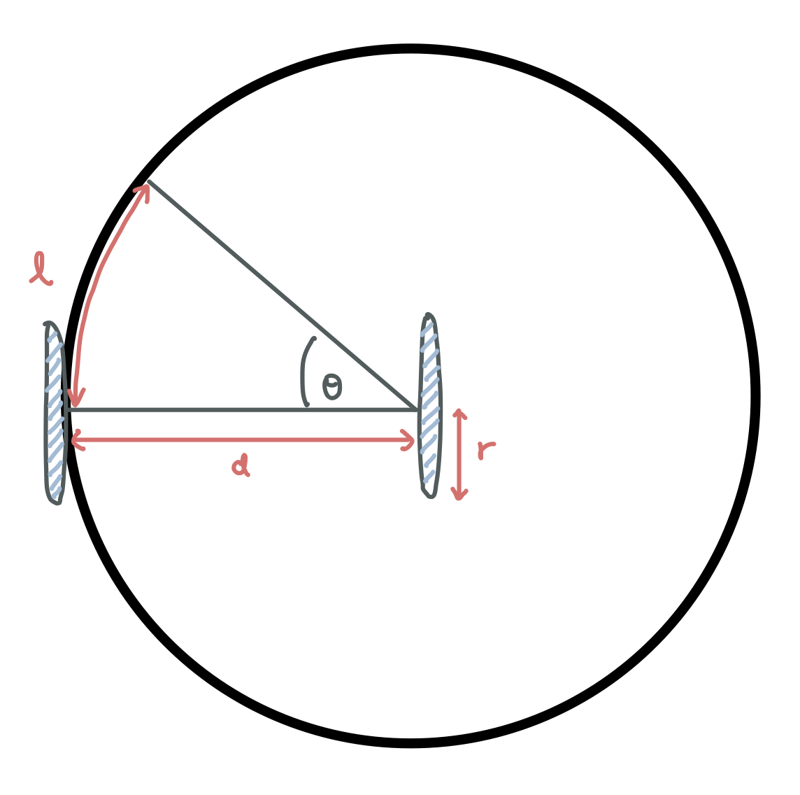
From the figure above, we can see that there are three labeled variables $l, d, r$. The variables $d$ corresponds to the width of the robot, and $r$ is radius of the wheel.
Let us define $s_l$ and $s_r$ to be the total distance traversed by the left wheel and total distance traversed by the right wheel respectively. These two variables can easily computed using the encoder measurements. The arc length $l$ equals to the difference $s_l - s_r$. The angle $\theta$ (in degrees) can be computed as shown below.
\[\theta = \frac{s_l - s_r}{d} \times \frac{180}{\pi} ^{\circ} = \frac{l}{d} \times \frac{180}{\pi} ^{\circ}\]From the simple model presented above, we can start implementing the the PID control for the robot’s current heading. The inputs would be $\phi_{set}$ and $\phi_{actual}$, where $\phi_{set}$ is the angle setpoint for the robot’s heading, whereas $\phi_{actual}$ is the robot’s actual heading.
The output range of the PID subVI block is set to $[-1, 1]$ and that would be used as the speed ratio, $r_{speed}$, to compute the output velocity to the left and right wheels. The variable $v_d$ is the desired velocity of the robot.
\[
\begin{aligned}
v_{left} & = v_d (1 + r_{speed}) \
v_{right} & = v_d (1 - r_{speed})
\end{aligned}
\]
4.3 Dead Reckoning
Determining robot (x, y) position and heading (theta) using encoders.
The dead reckoning of the robot was implemented with A Tutorial and Elementary Trajectory Model for the Differential Steering System of Robot Wheel Actuators by G.W. Lucas. The paper/tutorial was relatively easy to read and included various insights regarding the physical implementation and how the models were derived. “A Simpler Formula for Dead Reckoning” (Equation 6 on the tutorial page) was implemented and tested.
\[
\begin{aligned}
\bar{s} & = (s_R + s_L) \div 2 \
\theta & = (s_R - s_L) \div b + \theta_0 \
x & = \bar{s} cos(\theta) + x_0 \
y & = \bar{s} sin(\theta) + y_0
\end{aligned}
\]
$s_R$ and $s_L$ correspond to the right and left encoder distances, and $b$ is the width of the robot. $x_0$, $y_0$, $\theta_0$ are the corresponding initial values for position and angle.
The dead reckoning function would be called repeatedly as the robot is running, while the previous values $x_0$, $y_0$, $\theta_0$ are stored and passed into the function as inputs.
It is very important to note the points mentioned at the end of the tutorial page that for dead reckoning implementations, there is a limit on the accuracy of the computed values. If robot’s wheels encounter slippery surface or uneven surface, the wheels could slip and degrade the quality of measurement.
Even if the robot maintains traction, the position estimates are will vulnerable to backlash due to robot’s gearing and the inherent inaccuracies in the encoders and overall setup of the robot.
4.4 Kalman Filter
While the LiDAR interfacing operation was taking place, we decided to investigate the use of Kalman Filter so that we can use both the encoder and accelerometer measurements to compute the robot’s current position more accurately.
The resources we used for learning about Kalman Filter includes the built in examples in LabVIEW, which were interactive, helpful and relatively easy to understand. In addition, we also took some reference from Adam Shan’s blog post. Even though the blog post was written mainly in Chinese, it included some helpful illustration and equations which allowed us to see the bigger picture.
In the end, we were able to physically realise the CV (Constant Velocity) Model, and use the encoder and accelerometer measurements to compute the position and velocity of the robot.
\[\overrightarrow{x}(t) = (x \quad y \quad v_x \quad v_y)^T\] \[\overrightarrow{x}(t+\Delta t) = \left( \begin{array}{c} x(t) + \Delta t v_x \\ y(t) + \Delta t v_y \\ v_x \\ v_y \end{array} \right)\]
However, more complicated model such as CTRV (Constant Turn Rate and Velocity) Model requires Extended Kalman Filter for implementation, which is currently not included within the project scope. Nevertheless, we will continue to look into this possibility and conduct further research into Extended Kalman Filter and Unscented Kalman Filter.
4.5 Interfacing myRIO with LiDAR
This year, the NIARC team is very fortunate to be sponsored by SICK Australia, who provided us with the privilege of using a LiDAR (Light Detection And Ranging) sensor for obstacle detection and SLAM (Simultaneous Localisation And Mapping). We are grateful for the provided office tour/presentation, and their ongoing support for the provided hardware and software.
Important Prerequisites:
- SICK TIM571 LiDAR
- Ethernet (Female) to USB (Male) adapter
- NI-VISA and all relevant packages must be installed on myRIO, otherwise the NI-VISA related VI blocks would not work as expected. On the device we were working on, it was specifically
NI-VISA ENET Passportwhich had to be installed via NI MAX. - The ethernet-to-USB adapter needs to be plugged into the myRIO before the myRIO is turned on, otherwise the adapter would not be detected.
Steps for configuring the LiDAR with myRIO:
- Map the LiDAR IP address to what myRIO thinks it is on. We need to do this because myRIO does not do a proper network search for devices. (Or maybe we missed out on something and did not find the option to do so.)
- Change the TCP/IP setting on the LiDAR to match the IP address and subnet mask settings from the myRIO. Please see the example below, and notice that the LiDAR IP Address is modified slightly, from 161 to another number, in this case we used 170.
myRIO Network Information (check using NI MAX software)
IPV4 Address:   169.254.233.161
Subnet Mask:    255.255.0.0

LiDAR TCP/IP Settings (configure using SOPAS software)
IP Address:     169.254.233.170
Subnet Mask:    255.255.0.0
- Verify that the changes have been made to the LiDAR. In SOPAS,
SOPAS > TIM571 > Network > Ethernet > General, the updated settings should reflect the edited IP address which was written to the device. We could also usecmd > ipconfigtopingthe device and see whether it responds to the request. - Take note of the IP-Port from
SOPAS > Network > Ethernet > Ethernet Host Port > IP-Port, in this case we hadIP-Port: 2112. KeepCoLa Dialect: CoLa ASCIIas the selected option. - Connect the LiDAR to myRIO. If
sshis enabled on myRIO, we could check if myRIO can communicate with the LiDAR usingputtyandpingthe LiDAR. - In LabVIEW, we can use the following VISA subVIs:
VISA Open: create a constant for the VISA Resource Name withTCPIP::169.254.233.170::2112::SOCKET, and for Access Mode, useVISA Defaults.VISA Write: provide the command for Poll One Telegram. Ensure that thewrite bufferconstant provided is configured to Hex Display. Then from the Telegram Listing Manual, we can find that for Poll One Telegram, the corresponding Hex Command is02 73 52 4E 20 4C 4D 44 73 63 61 6E 64 61 74 61 03, then copy and paste that into thewrite bufferconstant.VISA Read: specify a sufficiently large number for the number of characters you want to read.VISA Close: used to close the the established connection.
- To parse the LiDAR data, follow the Telegram Structure specified in the TIM571 Technical Information Manual.
4.6 Obstacle Avoidance with LiDAR
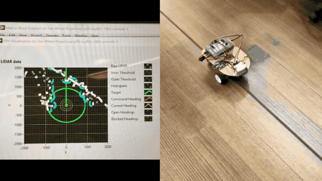
Obstacle avoidance with LiDAR was achieved through Simple VFH and Advanced VFH, where VFH is the abbreviation for (Vector Field Histogram).
The Simple VFH was used for initial testing, so that we could ensure the LiDAR was working as expected. The simple version “identifies obstacles and gaps, or open areas, in the robot environment, which you can use to implement reactionary motion in a robot vehicle”. However, it does not support goal-directed obstacle avoidance, and this is where the Advanced VFH comes in.
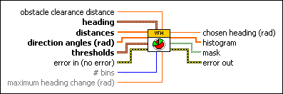
The Advanced VFH will avoid detected obstacles by searching for gaps/openings which are wide enough for the robot to pass through and direct the robot to specified goal position. In order for this VI to work, basic SLAM (Simultaneous Localisation and Mapping) implementation is required, so that we can keep track of $x, y, \theta$, which corresponds to the robot’s $(x,y)$ position and current heading $\theta$.
In the heading input, we provide the current robot heading and target heading. Distances and direction angles are directly provided by the LiDAR. Obstacle clearance distance basically defines the footprint of the robot body as a radius. Thresholds define the distances at which the robot considers itself blocked.
The GIF animation at the beginning of the blog post shows the Advanced VFH algorithm in action, and the left part specifically illustrates the RAW LiDAR data and the aforementioned settings and thresholds.
4.7 Finite State Machine
Once the Advanced VFH was implemented and tested, we moved on to defining waypoints using the good old finite state machine. This allowed us to easily manage the tasks and requirements specified for milestone 4.
What is next?
- Integrate Kalman Filter into the robot.
- Work towards completing the upcoming Milestone 5.